the ROOT tutorial plots, rebuilt — reference on the left, plotlyhep on the right
ROOT's df102_NanoAODDimuonAnalysis and df106_HiggsToFourLeptons tutorials draw the two canonical open-data plots. The right-hand figures are rebuilt from the tutorial sources — same selection and normalisation, same binning, canvas, fonts, label positions, colours — and compared pixel by pixel with the tutorial's own output on every commit (tests/compare_root.py). What the rebuild adds: hover a resonance label, a bin, a stack segment or a data point.
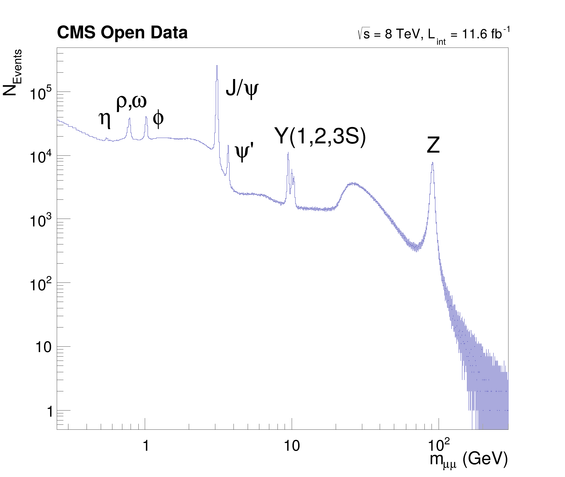
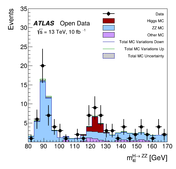
The 4ℓ selection is the tutorial's exact one (isolation, impact parameters, 25/15/10 GeV; ZZ × 1.3; 10 064 pb⁻¹; electron scale-factor variations for the hatched band), reduced by docs/make_data_root106.py; the dimuon spectrum is the tutorial's 30 000 uniform bins collapsed per pixel column the way ROOT's painter does it.
the same data in the plotlyhep template — H → ZZ* → 4ℓ, with controls
The four-lepton invariant mass after the standard selection (trigger (e or μ); exactly 4 leptons; Σcharge = 0; 4e, 4μ or 2e2μ; pT > 20, 15, 10 GeV (ROOT df106 tutorial)), Higgs signal stacked on the ZZ* and reducible backgrounds, data with Poisson errors. Built from CERN Open Data record 15005 with the normalisation of the ATLAS outreach framework; the same selection as ROOT's df106_HiggsToFourLeptons tutorial.
try: hover a stack segment · hover a data point (observed vs S and B) · channel dropdown · log axis · signal × 10 · click a legend entry to hide it. The figure is frozen; press edit (top right) to zoom, pan, drag the legend or move labels — your edits stay in this browser; reset discards them
Selected events: data 442 · MC after selection: ggH125_ZZ4lep 156360, VBFH125_ZZ4lep 181631, WH125_ZZ4lep 8842, ZH125_ZZ4lep 10526, llll 500088, Zee 160, Zmumu 161, ttbar_lep 249. Reduced once by docs/make_data.py to a 36 kB JSON; this page is built from that file alone.
the same data in the plotlyhep template — the dimuon spectrum, with controls
Every opposite-sign muon pair's invariant mass on a log–log axis: three decades of QCD and electroweak physics in one histogram, from the light mesons through the charmonium and bottomonium families to the Z. Hover a peak's label to learn what it is; hover a bin for its count; zoom to a family. 2012: CMS Open Data record 12341 — Run2012B+C DoubleMuParked, reduced to muons in NanoAOD format (8 TeV, 61.5 M events) · 2010: CMS Open Data record 700 — 100k dimuon events selected from the Run2010B Mu primary dataset (7 TeV).
try: hover the J/ψ or Υ labels · opposite- vs same-sign (no resonances in same-sign pairs: the peaks are physics, not detector artefacts) · zoom presets · frozen until you press edit, then drag to zoom or move the labels
main panel + ratio panel
php.ratio_figure("ATLAS", height_ratios=(3, 1), hspace=0.05) lays the two panels out exactly as matplotlib's GridSpec would (checked by the pixel harness against an mplhep figure), shares the x axis, and php.ratioplot(fig, data, mc, bins, den_w2=…) draws data / MC with its errors, the MC statistical band around one, and the dashed reference line. Hover a ratio point for the numbers behind it. open in editor
use it
import plotlyhep as php
fig = php.figure("ATLAS", barmode="stack", bargap=0)
fig.add_trace(go.Bar(x=centres, y=yields, width=widths, name="ZZ*", customdata=per_bin_html, hovertemplate="%{customdata}<extra></extra>"))
php.atlas.label(fig, "Open Data", data=True, lumi=10, com=13, loc=1)
php.set_xlabel(fig, "m<sub>4ℓ</sub> [GeV]"); php.set_ylabel(fig, "Events / 3.75 GeV")

# in an HTML deck: once per page, then per figure
head  += php.html.script_tag("ATLAS") + php.html.SLIDE_CSS
slide += php.html.embed(fig, "plot-s12")                     # frozen: hover + buttons only; the "edit" chip unlocks dragging, zoom, persisted edits
Fidelity to mplhep is measured, not asserted: every commit renders the same figures through mplhep and plotlyhep on a 1000 × 1000 grid and diffs the pixels — see the pixel-diff workflow and the README table.